Forced Damped Oscillations
This applet shows the solution(s) for an oscillating system, with damping and a forcing function. The behavior of the displacement variable "x" with time "t" is defined by the second-order linear ordinary differential equation (ODE):
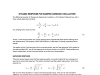
D[x,t,2] + alpha*D[x,t,1] + beta*x = F*Cos(gamma*t)
where D[x,t,n] represents the derivative of the displacement variable x with respect to time t, of order "n". The damping term alpha*D[x,t,1] assumes a velocity-dependent damping force (often called "viscous" damping); this is NOT friction.
The time-dependent response x(t) has two parts: (1) the response to the initial conditions (IC) of the system, which are the initial displacement and initial velocity, and (2) the response to the driving function. Since these solutions are independent, the overall solution for the ODE is just the superposition (sum) of both.
Here is a summary of the controls on the applet: "alph" is the damping constant alpha; "bet" is the restoring force parameter beta; "x0" is the initial displacement (at time zero); "v0" is the initial velocity; "F" is the amplitude of the driving function; "gama" is the parameter that controls the frequency of the driving function. There are four checkboxes, to enable/disable the plotting of the indicated responses.
There are two numerical values displayed: "zeta" is the damping ratio (an important parameter that affects the solution shape), and "omega" is the natural, unforced, frequency of the system. The damping ratio is
zeta = alpha / ( 2 Sqrt(beta) )
and this expresses the relative strengths of the damping and restoring forces.
There is a slider to adjust the number of steps used in the plotting; use a smaller number like 200 to more quickly see the general behavior, then increase "nsteps" as needed to refine the plotting (make the curves smoother).
With this many parameters to adjust, of course many solution scenarios are possible. Here are a few cases, to begin explorations.
(1) Disable all response plots other than the "free" response. Make the following settings: alpha=0, beta=1.65, x0=10, v0=0, F=0, gamma=0. Sweep beta back and forth by selecting its slider, then use the arrow keys. Observe the frequency changing on the plot, and omega changing.
(2) Reset beta to 1.65, then select the v0 slider. Observe the response as you increase and decrease v0; include some negative values. Change x0 as well, to see that the motion can begin from any x value, including zero (the equilibrium position).
(3) Reset v0=0 and x0=10; select the alpha slider. Use the arrow keys to increase alpha, observe the effect of damping. Notice zeta changing, and that omega also changes.
(4) A special case is called "critical damping." To set this up, use alpha=1, beta=0.25, x0=15, v0=0, F=0, gamma=0. Notice that zeta is 1, and omega is 0; the latter is because the motion is not periodic.
(5) Uncheck the free response plot, enable the forced response plot. Set alpha=0.06, beta=1.65, x0=15, v0=0, F=8, gamma=1. Enable the forcing function plot. Select the beta slider, use the arrow keys to vary beta; observe the variation in the forced response. Notice the value of omega as beta varies; when omega is close to 1, the forced response is very large. This condition, when the forcing frequency gamma equals the natural frequency omega of the system, is called "resonance."