Images to applet: Generating two different uniformly distributed points on a sphere from another uniform distribution.
This applet contains images and explanations of the results of applet: Generating two different uniformly distributed points on a sphere from another uniform distribution.
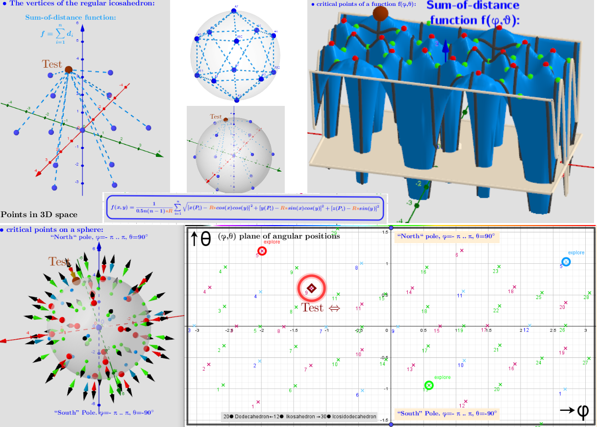
Some initial uniform distribution is taken -icosahedron with 12 vertices. The function of the sum of distances f(φ, θ) is considered -the sum of all distances from any point on the sphere (R;φ;θ) to the points of the selected initial distribution (the spherical coordinate system is used). Using Lagrange multipliers, the critical points of the distance sum function subject to a constraining equation g(x,y,z)=x²+y²+z²-R² are found. There is a system of equations: ∇f(x,y,z)= λ∇g(x,y,z). A local optimum occurs when ∇f(x,y,z) and ∇g(x,y,z) are parallel, and so ∇f is some multiple of ∇g.
The vertices of the polyhedra are considered as 3 subsets of the 3 types of critical points for the distance sum function f(φ, θ). It should be noted that the angular positions of the points of the original distribution and the obtained local minima coincide.
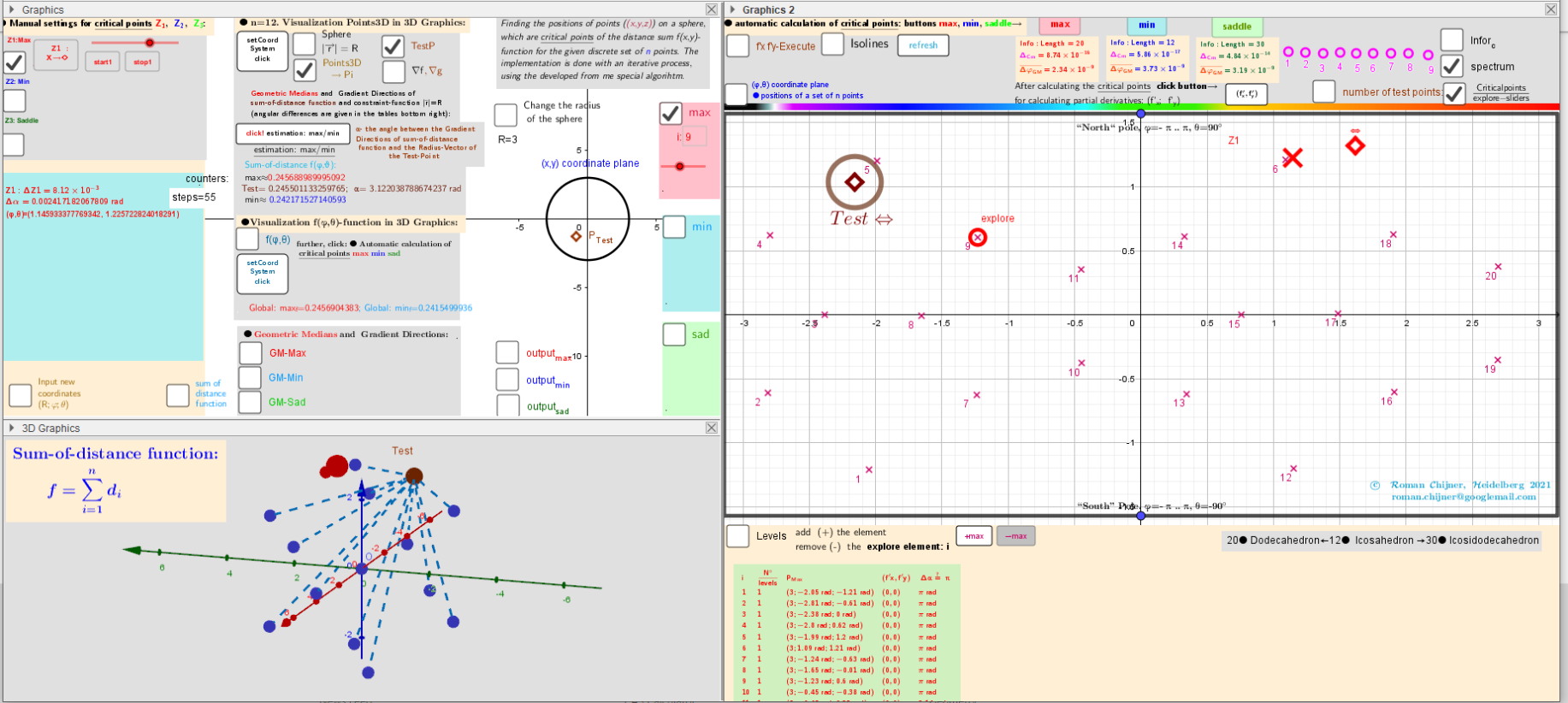
Finding critical points is realized by using three different schemes separately for each type of critical points. The visualization of the solutions, founded by iterative methods, is carried out using the corresponding graphs of partial derivatives and level lines by which one can judge the type of critical points. The accuracy of the solutions that were found is controlled by the calculated values of the angles between the vectors ∇f and ∇g tends to π. The data are summarized in the tables.
It should be noted that automatic calculation of critical points (click buttons max, min, saddle) does not always find all solutions. In manual mode (Manual settings for critical points), these inaccuracies can be corrected with the available tools: remove/add solutions: add (+) and remove ( - ) the elements. Levels are the values of f(φ, θ) for critical points. Above coordinate plane (φ, θ) you will find the number of critical points of each type, means of sum of all correction angles of geometric medians (GM):ΔφGM and geometric centers (GC):ΔφCM -angular deviations from directions of the corresponding position vectors. For visibility, we denote polyhedra that have in the case of ΔφGM→0: as ● otherwise as ☐.
The uniform distribution of icosahedron points "induces" on the surface of the sphere critical points (found using Lagrange multipliers) of the Sum-of-distance function.
Applet image.
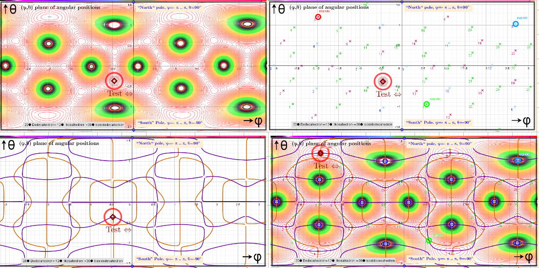
Isolines, Critical points, implicit functions of partial differential equations equal to zero over a rectangular region: - π ≤φ ≤ π; -π/2≤θ≤π/2. Test point -a colored moveable indicator of the critical point type.
A critical points scheme for Generating uniformly distributed points on a sphere.
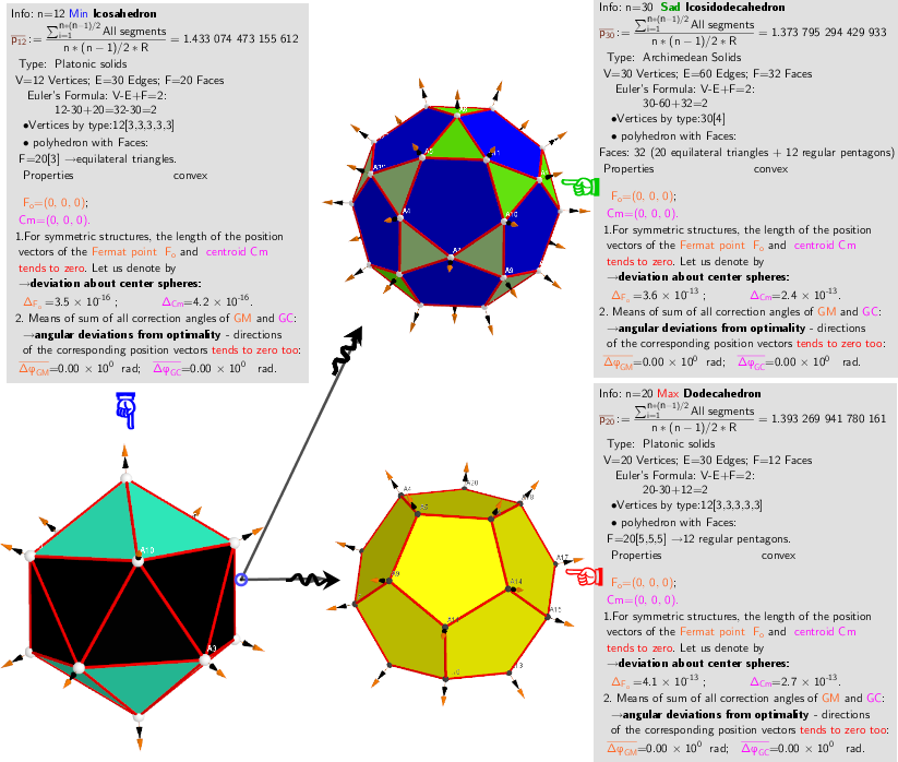
Vertices of a polyhedra as subsets of critical points of the sum-of-distances function f(φ,θ).
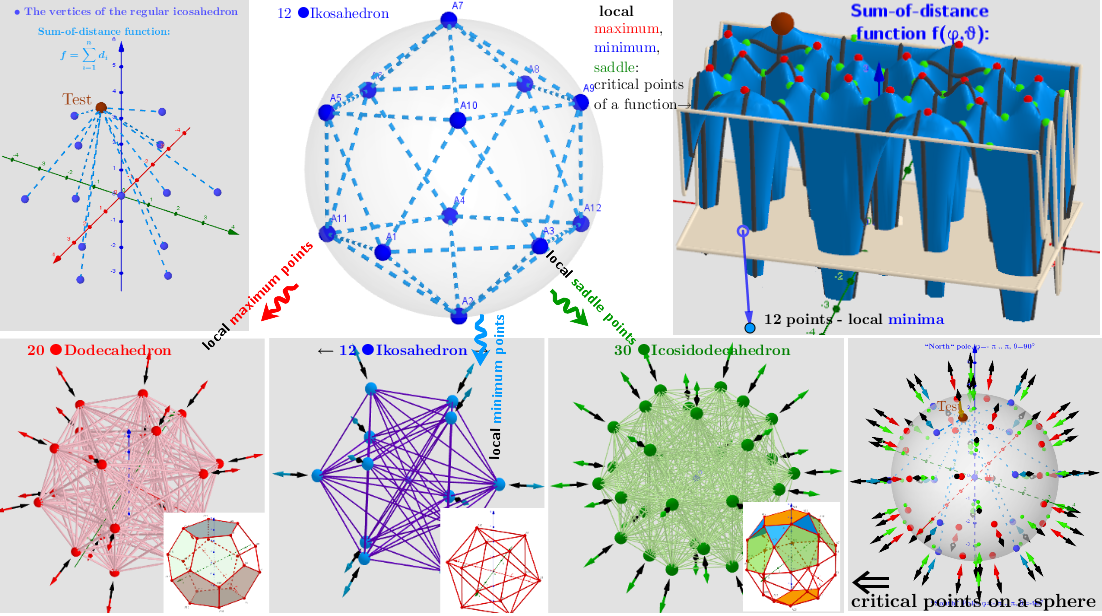
20 ●Dodecahedron← 12 ●Icosahedron →30 ●Icosidodecahedron.